MATH 204 Introduction to Statistics
Lecture 12: Further Inference
JMG
Goals for Lecture
- In this lecture, we introduce statistical inference for
Goals for Lecture
In this lecture, we introduce statistical inference for
- a single proportion (6.1)
Goals for Lecture
In this lecture, we introduce statistical inference for
a single proportion (6.1)
a difference of two proportions (6.2)
Goals for Lecture
In this lecture, we introduce statistical inference for
a single proportion (6.1)
a difference of two proportions (6.2)
one-sample means (7.1)
Goals for Lecture
In this lecture, we introduce statistical inference for
a single proportion (6.1)
a difference of two proportions (6.2)
one-sample means (7.1)
paired data (7.3)
Goals for Lecture
In this lecture, we introduce statistical inference for
a single proportion (6.1)
a difference of two proportions (6.2)
one-sample means (7.1)
paired data (7.3)
a difference of two means (7.3)
Goals for Lecture
In this lecture, we introduce statistical inference for
a single proportion (6.1)
a difference of two proportions (6.2)
one-sample means (7.1)
paired data (7.3)
a difference of two means (7.3)
After we discuss these topics along with power calculations and simple ordinary least squares regression (7.4 and Chapter 8), we will return to discuss goodness of fit (6.3) and testing for independence (6.4).
Learning Objectives
- After this lecture, you should be able to conduct and apply point estimates, interval estimates, and hypothesis tests for
Learning Objectives
After this lecture, you should be able to conduct and apply point estimates, interval estimates, and hypothesis tests for
- proportions, difference of proportions, one sample means, paired data, and difference of two means.
Learning Objectives
After this lecture, you should be able to conduct and apply point estimates, interval estimates, and hypothesis tests for
- proportions, difference of proportions, one sample means, paired data, and difference of two means.
This includes knowing when to use which type of hypothesis test, and
what is the appropriate R command(s) to use.
Many of our interval estimates and hypothesis tests will rely on a central limit theorem. We quickly review these.
Central Limit Theorems
- Recall our CLT for sample proportions:
When observations are independent and sample size is sufficiently large, then the sampling distribution for the sample proportion ˆp^p is approximately normal with mean μˆp=p and standard error SEˆp=√p(1−p)n.
Central Limit Theorems
- Recall our CLT for sample proportions:
When observations are independent and sample size is sufficiently large, then the sampling distribution for the sample proportion ˆp is approximately normal with mean μˆp=p and standard error SEˆp=√p(1−p)n.
- We also have a CLT for the sample mean:
When we collect samples of sufficiently large size n from a population with mean μ and standard deviation σ, then the sampling distribution for the sample mean ˉx is approximately normal with mean μˉx=μ and standard error SEˉx=σ√n.
- Later we will return to discuss precisely what we mean by "samples of sufficiently large size."
- We use sampling distributions for obtaining confidence intervals and conducting hypothesis tests.
Videos for CLT
- Central limit theorems are reviewed in the videos included on the next few slides.
CLT Video 1
CLT Video 2
CLT Video 3
CI for a Proportion
- Once you've determined a one-proportion CI would be helpful for an application, there are four steps to constructing the interval:
CI for a Proportion
Once you've determined a one-proportion CI would be helpful for an application, there are four steps to constructing the interval:
- Identify the point estimate ˆp and the sample size n, and determine what confidence level you want.
CI for a Proportion
Once you've determined a one-proportion CI would be helpful for an application, there are four steps to constructing the interval:
Identify the point estimate ˆp and the sample size n, and determine what confidence level you want.
Verify the conditions to ensure ˆp is nearly normal, that is, check that nˆp≥10 and n(1−ˆp)≥10.
If the conditions hold, estimate the standard error SE using ˆp, find the appropriate z∗, and compute ˆp±z∗×SE .
Interpret the CI in the context of the problem.
Proportion CI Example
- Consider the following problem:
Proportion CI Example
- Consider the following problem:
Is parking a problem on campus? A randomly selected group of 89 faculty and staff are asked whether they are satisfied with campus parking or not. Of the 89 individuals surveyed, 23 indicated that they are satisfied. What is the proportion p of faculty and staff that are satisfied with campus parking?
- Explain why this problem is suitable for a one-proportion CI. Is this CLT applicable? If so, obtain a 95% CI for a point estimate.
Proportion CI Video
- Confidence intervals for a proportion are reviewed in this video:
Hypothesis Test for a Proportion
- Once you've determined a one-proportion hypothesis test is the correct test for a problem, there are four steps to completing the test:
Hypothesis Test for a Proportion
Once you've determined a one-proportion hypothesis test is the correct test for a problem, there are four steps to completing the test:
- Identify the parameter of interest, list hypotheses, identify the significance level, and identify ˆp and n.
Hypothesis Test for a Proportion
Once you've determined a one-proportion hypothesis test is the correct test for a problem, there are four steps to completing the test:
Identify the parameter of interest, list hypotheses, identify the significance level, and identify ˆp and n.
Verify conditions to ensure ˆp is nearly normal under H0. For one-proportion hypothesis tests, use the null value p0 to check the conditions np0≥10 and n(1−p0)≥10.
If the conditions hold, compute the standard error, again using p0, compute the Z-score, and identify the p-value.
Evaluate the hypothesis test by comparing the p-value to the significance level α, and provide a conclusion in the context of the problem.
Hypotheses for One Proportion Tests
- The null hypothesis for a one-proportion test is typically stated as H0:p=p0 where p0 is a hypothetical value for p.
Hypotheses for One Proportion Tests
The null hypothesis for a one-proportion test is typically stated as H0:p=p0 where p0 is a hypothetical value for p.
The corresponding alternative hypothesis is then one of
Hypotheses for One Proportion Tests
The null hypothesis for a one-proportion test is typically stated as H0:p=p0 where p0 is a hypothetical value for p.
The corresponding alternative hypothesis is then one of
- HA:p≠p0 (two-sided),
Hypotheses for One Proportion Tests
The null hypothesis for a one-proportion test is typically stated as H0:p=p0 where p0 is a hypothetical value for p.
The corresponding alternative hypothesis is then one of
HA:p≠p0 (two-sided),
HA:p<p0 (one-sided less than), or
Hypotheses for One Proportion Tests
The null hypothesis for a one-proportion test is typically stated as H0:p=p0 where p0 is a hypothetical value for p.
The corresponding alternative hypothesis is then one of
HA:p≠p0 (two-sided),
HA:p<p0 (one-sided less than), or
HA:p>p0 (one-sided greater than)
Proportion Hypothesis Test Example
Is parking a problem on campus? A randomly selected group of 89 faculty and staff are asked whether they are satisfied with campus parking or not. Of the 89 individuals surveyed, 23 indicated that they are satisfied.
Proportion Hypothesis Test Example
Is parking a problem on campus? A randomly selected group of 89 faculty and staff are asked whether they are satisfied with campus parking or not. Of the 89 individuals surveyed, 23 indicated that they are satisfied.
- Let's study this problem using a hypothesis testing framework.
- Here is relevant R code:
## [1] 44.5 44.5## [1] -4.557991## [1] 5.164528e-06p_hat <- 23/89n <- 89p0 <- 0.5(c(n*p0,n*(1-p0))) # success-failure conditionSE <- sqrt((p0*(1-p0))/n)(z_val <- (p_hat - p0)/SE)(p_value <- 2*(pnorm(z_val)))R Command(s) for Proportion Hypothesis Test
- In cases where the CLT applies, we can use a normal distribution to directly compute p-values with the
pnormfunction.
R Command(s) for Proportion Hypothesis Test
In cases where the CLT applies, we can use a normal distribution to directly compute p-values with the
pnormfunction.Alternatively, R has a built-in function
prop.testthat automates one-proportion hypothesis testing.
R Command(s) for Proportion Hypothesis Test
In cases where the CLT applies, we can use a normal distribution to directly compute p-values with the
pnormfunction.Alternatively, R has a built-in function
prop.testthat automates one-proportion hypothesis testing.So, in our parking problem example we would use
## ## 1-sample proportions test without continuity correction## ## data: 23 out of 89, null probability 0.5## X-squared = 20.775, df = 1, p-value = 5.165e-06## alternative hypothesis: true p is not equal to 0.5## 95 percent confidence interval:## 0.1788154 0.3580294## sample estimates:## p ## 0.258427prop.test(23,89,p=0.5,correct = FALSE)Problems to Practice
- Let's take a minute to do some practice problems.
Problems to Practice
Let's take a minute to do some practice problems.
Try problems 6.7 and 6.13 from the textbook.
Problems Involving Difference of Proportions
- Consider the following problem:
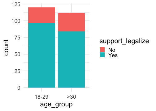
An online poll on January 10, 2017 reported that 97 out of 120 people in Virginia between the ages of 18 and 29 believe that marijuana should be legal, while 84 out of 111 who are 30 and over held this belief. Is there a difference between the proportion of young people who favor marijuana leagalization as compared to people who are older?
Problems Involving Difference of Proportions
- Consider the following problem:
An online poll on January 10, 2017 reported that 97 out of 120 people in Virginia between the ages of 18 and 29 believe that marijuana should be legal, while 84 out of 111 who are 30 and over held this belief. Is there a difference between the proportion of young people who favor marijuana leagalization as compared to people who are older?
- Think about how this problem is different than problems for a single proportion. The basic point here is that there are two groups, and we want to compare proportions across the two groups.
- Data for the problem stated above might look as follows (only the first few rows are shown).
## # A tibble: 6 × 2## support_legalize age_group## <chr> <fct> ## 1 Yes >30 ## 2 No 18-29 ## 3 Yes >30 ## 4 Yes >30 ## 5 Yes >30 ## 6 Yes 18-29Plotting Grouped Proportion Data
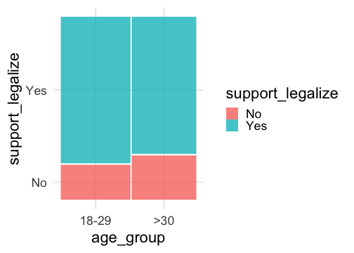
- We can used grouped bar plots or a mosaic plot to visualize data related to grouped proportions:
Sampling Distribution for Difference of Proportions
The difference ˆp1−ˆp2 can be modeled using a normal distribution when
The data are independent within and between the two groups. Generally this is satisfied if the data come from two independent random samples or if the data come from a randomized experiment.
The success-failure condition holds for both groups, where we check successes and failures in each group separately.
- When these conditions are satisfied, the standard error of ˆp1−ˆp2 is
SE=√p1(1−p1)n1+p2(1−p2)n2, where p1 and p2 represent the population proportions, and n1 and n2 represent the sample sizes.
CI for Difference of Proportions
- To construct a CI for a difference of proportion, we can apply the formulas
SE=√p1(1−p1)n1+p2(1−p2)n2, CI=point estimate±z∗×SE
CI for Difference of Proportions
- To construct a CI for a difference of proportion, we can apply the formulas
SE=√p1(1−p1)n1+p2(1−p2)n2, CI=point estimate±z∗×SE
- If necessary, we can use the plug-in principle to estimate the standard error.
SE≈√ˆp1(1−ˆp1)n1+ˆp2(1−ˆp2)n2
CI for Difference of Proportions Examples
- Let's obtain a 90% CI for the difference of proportions in the marijuana legalization question. Here is the relevant R code:
## [1] 97 23 84 27## [1] -0.03775321 0.14090636n1 <- 120n2 <- 111p1 <- 97/n1p2 <- 84/n2p_diff <- p1 - p2(c(n1*p1,n1*(1-p1),n2*p2,n2*(1-p2))) # success-failure conditionsSE <- sqrt(((p1*(1-p1))/n1) + ((p2*(1-p2))/n2))z_90 <- -qnorm(0.05) # find the appropriate z-value for 90% CI(CI <- p_diff + z_90 * c(-1,1) * SE) # 90% CICI for Difference of Proportions Examples
- Let's obtain a 90% CI for the difference of proportions in the marijuana legalization question. Here is the relevant R code:
## [1] 97 23 84 27## [1] -0.03775321 0.14090636n1 <- 120n2 <- 111p1 <- 97/n1p2 <- 84/n2p_diff <- p1 - p2(c(n1*p1,n1*(1-p1),n2*p2,n2*(1-p2))) # success-failure conditionsSE <- sqrt(((p1*(1-p1))/n1) + ((p2*(1-p2))/n2))z_90 <- -qnorm(0.05) # find the appropriate z-value for 90% CI(CI <- p_diff + z_90 * c(-1,1) * SE) # 90% CI- Let's try some more examples together.
Hypotheses for Difference of Proportion Tests
- The null hypothesis for a difference of proportions test is typically stated as H0:p1−p2=p0 where p0 is a hypothetical value for p.
Hypotheses for Difference of Proportion Tests
The null hypothesis for a difference of proportions test is typically stated as H0:p1−p2=p0 where p0 is a hypothetical value for p.
The corresponding alternative hypothesis is then one of
Hypotheses for Difference of Proportion Tests
The null hypothesis for a difference of proportions test is typically stated as H0:p1−p2=p0 where p0 is a hypothetical value for p.
The corresponding alternative hypothesis is then one of
- HA:p1−p2≠p0 (two-sided),
Hypotheses for Difference of Proportion Tests
The null hypothesis for a difference of proportions test is typically stated as H0:p1−p2=p0 where p0 is a hypothetical value for p.
The corresponding alternative hypothesis is then one of
HA:p1−p2≠p0 (two-sided),
HA:p1−p2<p0 (one-sided less than), or
Hypotheses for Difference of Proportion Tests
The null hypothesis for a difference of proportions test is typically stated as H0:p1−p2=p0 where p0 is a hypothetical value for p.
The corresponding alternative hypothesis is then one of
HA:p1−p2≠p0 (two-sided),
HA:p1−p2<p0 (one-sided less than), or
HA:p1−p2>p0 (one-sided greater than)
When p0=0 we need to use the pooled proportion.
Pooled Proportion
- When the null hypothesis is that the proportions are equal, use the pooled proportion ˆppooled, where
ˆppooled=number of "successes"number of cases=ˆp1n1+ˆp2n2n1+n2
Pooled Proportion
- When the null hypothesis is that the proportions are equal, use the pooled proportion ˆppooled, where
ˆppooled=number of "successes"number of cases=ˆp1n1+ˆp2n2n1+n2
- The pooled proportion ˆppooled is used to check the success-failure condition and to estimate the standard error.
Hypothesis Test for Difference of Proportions
- Let's apply the hypothesis testing framework to this problem:
An online poll on January 10, 2017 reported that 97 out of 120 people in Virginia between the ages of 18 and 29 believe that marijuana should be legal, while 84 out of 111 who are 30 and over held this belief. Is there a difference between the proportion of young people who favor marijuana leagalization as compared to people who are older?
## [1] 69.73593 19.26407## [1] 0.9510127## [1] 0.3415979n1 <- 120; n2 <- 111p1 <- 97/120; p2 <- 84/111; p_diff <- p1 - p2p_pooled <- (p1*n1+p2*n2)/(n1+n2)(c(n*p_pooled,n*(1-p_pooled)))SE <- sqrt((p_pooled*(1-p_pooled))/n1 + (p_pooled*(1-p_pooled))/n2)(z_val <- (p_diff - 0.0)/SE)(p_value <- 2*(1-pnorm(z_val)))R Commands for Difference of Proportion Test
- The R command
prop.testalso works for testing a difference of proportions.
R Commands for Difference of Proportion Test
The R command
prop.testalso works for testing a difference of proportions.For example, we could solve the marijuana legalization problem with the following:
## ## 2-sample test for equality of proportions without continuity correction## ## data: c(97, 84) out of c(120, 111)## X-squared = 0.90443, df = 1, p-value = 0.3416## alternative hypothesis: two.sided## 95 percent confidence interval:## -0.05486643 0.15801958## sample estimates:## prop 1 prop 2 ## 0.8083333 0.7567568prop.test(c(97,84),c(120,111),correct = FALSE)Hypothesis Test for Difference of Proportions Examples
- Let's work some more problems together.
Inference for a Sample Mean
- A potato chip manufacturer claims that there is on average 32 chips per bag for their brand. How can we tell if this is an accurate claim?
Inference for a Sample Mean
A potato chip manufacturer claims that there is on average 32 chips per bag for their brand. How can we tell if this is an accurate claim?
One approach is to take a sample of, say 25 bags of chips for the particular band and compute the sample mean number of chips per bag.
This type of problem is inference for a sample mean.
In principle, we know the sampling distribution for the sample mean is very nearly normal, provided the conditions for the CLT holds.
One question is, what are the appropriate conditions to check to make sure the CLT holds for the sample mean?
When the conditions for the CLT for the sample mean hold, the expression for the standard error involves the population standard deviation ( σ ) which we rarely know if practice. So, how do we estimate the standard error for the sample mean?
We address these questions in the next few slides.
Inference for a Mean Video
- You are encouraged to watch this video on inference for a mean.
Conditions for CLT for Sample Mean
- Two conditions are required to apply the CLT for a sample mean ˉx:
Conditions for CLT for Sample Mean
- Two conditions are required to apply the CLT for a sample mean ˉx:
Independence: The sample observations must be independent. Simple random samples from a population are independent, as are data from a random process like rolling a die or tossing a coin.
Conditions for CLT for Sample Mean
- Two conditions are required to apply the CLT for a sample mean ˉx:
Independence: The sample observations must be independent. Simple random samples from a population are independent, as are data from a random process like rolling a die or tossing a coin. Normality: When a sample is small, we also require that the sample observations come from a normally distributed population. This condition can be relaxed for larger sample sizes.
- The normality condition is vague but there are some approximate rules that work well in practice.
Practical Check for Normality
- n<30: If the sample size n is less than 30 and there are no clear outliers, then we can assume the data come from a nearly normal distribution.
Practical Check for Normality
n<30: If the sample size n is less than 30 and there are no clear outliers, then we can assume the data come from a nearly normal distribution.
n≥30: If the sample size n is at least 30 and there are no particularly exterme outliers, then we can assume the sampling distribution of ˉx is nearly normal, even if the underlying distribution of individual observations is not.
Let's consider example 7.1 from the textbook to illustrate these practical rules.
Estimating Standard Error
- When samples are independent and the normality condition is met, then the sampling distribution for the sample mean ˉx is (very nearly) normal with mean μˉx=μ and standard error SEˉx=σ√n, where μ is the true population mean of the distribution from which the samples are taken and σ is the true population from which the samples are taken.
Estimating Standard Error
When samples are independent and the normality condition is met, then the sampling distribution for the sample mean ˉx is (very nearly) normal with mean μˉx=μ and standard error SEˉx=σ√n, where μ is the true population mean of the distribution from which the samples are taken and σ is the true population from which the samples are taken.
In practice we do not know the true values of the population parameters μ and σ. But we can use the plug-in principle to obtain estimates:
μˉx≈ˉx, and SEˉx≈s√n,
where s is the sample standard deviation.
T-score
- If we take n samples from a normal distribution N(μ,σ), then the quantity
z=ˉx−μσ√n will follow a standard normal distribution N(0,1).
T-score
- If we take n samples from a normal distribution N(μ,σ), then the quantity
z=ˉx−μσ√n will follow a standard normal distribution N(0,1).
- On the other hand, the quantity
t=ˉx−μs√n will not quite be N(0,1), especially if n is small.
T-score
- If we take n samples from a normal distribution N(μ,σ), then the quantity
z=ˉx−μσ√n will follow a standard normal distribution N(0,1).
- On the other hand, the quantity
t=ˉx−μs√n will not quite be N(0,1), especially if n is small.
- We call the quantity in the last formula a T-score.
T-Score Video
- Let's watch this video on T-scores.
t-distribution
- T-scores follow a t-distribution with degrees of freedom df=n−1, where n is the sample size.
t-distribution
T-scores follow a t-distribution with degrees of freedom df=n−1, where n is the sample size.
We will use t-distributions for inference, that is, for obtaining confidence intervals and hypothesis testing.
t-distribution
T-scores follow a t-distribution with degrees of freedom df=n−1, where n is the sample size.
We will use t-distributions for inference, that is, for obtaining confidence intervals and hypothesis testing.
Let's get a feel for t-distributions.
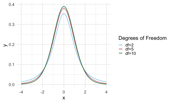
Degrees of Freedom Parameter
- This plot shows three different t density functions for three different degrees of freedom:
A Computational Experiment
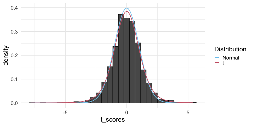
- This plot shows a histogram of T-score values obtained by computing the sample mean with n=8 from N(0,1). We overlay a density curve for both N(0,1) and a t-distribution with df=7:
Area Under a t-Distribution
- We can compute areas under t-distribution density curves in the same way we did for areas under normal distribution density curves. For example, the area
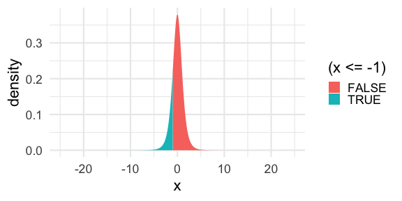
is computed by
pt(-1.0,df=5)## [1] 0.1816087Middle 95% Under a t Density
- How do we find the middle 95% of area under a t-distribution? This is an important question because it relates to construting a 95% confidence interval for the sample mean.
Middle 95% Under a t Density
How do we find the middle 95% of area under a t-distribution? This is an important question because it relates to construting a 95% confidence interval for the sample mean.
Suppose we have a t-distribution with degrees of freedom df=10, then to find the value t∗ so that 95% of the area under the density curve lies between −t∗ and t∗, we use the
qtcommand, for example,
- We can check our answer:
- Note that you always have to specify the appropriate value for the degrees of freedom df. The appropriate degrees of freedom is given by df=n−1, where n is the sample size.
One-Sample t CI
Based on a sample of n independent and nearly normal observations, a confidence interval for the population mean is ˉx±t∗df×s√n,
where n is the sample size, ˉx is the sample mean, s is the sample standard deviation.
One-Sample t CI
Based on a sample of n independent and nearly normal observations, a confidence interval for the population mean is ˉx±t∗df×s√n,
where n is the sample size, ˉx is the sample mean, s is the sample standard deviation.
- We determine the appropriate value for t∗df with the R command
qt((1.0-confidence_level)/2,df=n-1).
One-Sample Mean CI Example
- Suppose we take a random sample of 13 observations from a normally distributed population and determine the sample mean is 8 with a sample standard deviation of 2.5. Then to find a 90% confidence interval, we would do the following:
## [1] 6.764206 9.235794n <- 13x_bar <- 8s <- 2.5SE <- s/sqrt(n)t_ast <- -qt((1.0-0.9)/2,df=n-1)(CI <- x_bar + t_ast * c(-1,1)*SE)A 95% CI would be
## [1] 6.489265 9.510735t_ast <- -qt((1.0-0.95)/2,df=n-1)(CI <- x_bar + t_ast * c(-1,1)*SE)CI for Single Mean Summary
Once you have determined a one-mean confidence interval would be helpful for an application, there are four steps to constructing the interval:
CI for Single Mean Summary
Once you have determined a one-mean confidence interval would be helpful for an application, there are four steps to constructing the interval:
- Identify n, ˉx, and s, and determine what confidence level you wish to use.
CI for Single Mean Summary
Once you have determined a one-mean confidence interval would be helpful for an application, there are four steps to constructing the interval:
- Identify n, ˉx, and s, and determine what confidence level you wish to use.
- Verify the conditions to ensure ˉx is nearly normal.
CI for Single Mean Summary
Once you have determined a one-mean confidence interval would be helpful for an application, there are four steps to constructing the interval:
- Identify n, ˉx, and s, and determine what confidence level you wish to use.
Verify the conditions to ensure ˉx is nearly normal.
If the conditions hold, approximate SE by s√n, find t∗df, and construct the interval.
Interpret the confidence interval in the context of the problem.
One-Mean Hypothesis Testing
- The null hypothesis for a one-proportion test is typically stated as H0:μ=μ0 where μ0 is the null value for the population mean.
One-Mean Hypothesis Testing
The null hypothesis for a one-proportion test is typically stated as H0:μ=μ0 where μ0 is the null value for the population mean.
The corresponding alternative hypothesis is then one of
One-Mean Hypothesis Testing
The null hypothesis for a one-proportion test is typically stated as H0:μ=μ0 where μ0 is the null value for the population mean.
The corresponding alternative hypothesis is then one of
- HA:μ≠μ0 (two-sided),
One-Mean Hypothesis Testing
The null hypothesis for a one-proportion test is typically stated as H0:μ=μ0 where μ0 is the null value for the population mean.
The corresponding alternative hypothesis is then one of
HA:μ≠μ0 (two-sided),
HA:μ<μ0 (one-sided less than), or
One-Mean Hypothesis Testing
The null hypothesis for a one-proportion test is typically stated as H0:μ=μ0 where μ0 is the null value for the population mean.
The corresponding alternative hypothesis is then one of
HA:μ≠μ0 (two-sided),
HA:μ<μ0 (one-sided less than), or
HA:μ>μ0 (one-sided greater than)
One-Mean Hypothesis Test Procedure
- Once you have determined a one-mean hypothesis test is the correct procedure, there are four steps to completing the test:
One-Mean Hypothesis Test Procedure
Once you have determined a one-mean hypothesis test is the correct procedure, there are four steps to completing the test:
- Identify the parameter of interest, list out hypotheses, identify the significance level, and identify n, ˉx, and s.
One-Mean Hypothesis Test Procedure
Once you have determined a one-mean hypothesis test is the correct procedure, there are four steps to completing the test:
Identify the parameter of interest, list out hypotheses, identify the significance level, and identify n, ˉx, and s.
Verify conditions to ensure ˉx is nearly normal.
If the conditions hold, approximate SE by s√n, compute the T-score using
T=ˉx−μ0s√n, and compute the p-value.
- Evaluate the hypothesis test by comparing the p-value to the significance level α, and provide a conclusion in the context of the problem.
A Simple Example
- We want to know if the following data comes from a normal distribution with mean 0:
## [1] -0.36047565 -0.03017749 1.75870831 0.27050839 0.32928774 1.91506499## [7] 0.66091621 -1.06506123 -0.48685285 -0.24566197- We can apply a hypothesis test corresponding to H0:μ=0.0, versus HA:μ≠0 as follows
## [1] 0.9105232## [1] 0.3862831n <- length(x); x_bar <- mean(x); s <- sd(x)alpha <- 0.05SE <- s/sqrt(n)mu_0 <- 0.0(T <- (x_bar - mu_0)/SE)(p_value <- 2*(1-pt(T,df=n-1)))R Command for One-Sample t-test
- There is a built-in R command,
t.testthat will conduct a hypothesis test for a sinlg emean for us.
R Command for One-Sample t-test
There is a built-in R command,
t.testthat will conduct a hypothesis test for a sinlg emean for us.For example, we can solve our previous problem using
## ## One Sample t-test## ## data: x## t = 0.91052, df = 9, p-value = 0.3863## alternative hypothesis: true mean is not equal to 0## 95 percent confidence interval:## -0.4076704 0.9569217## sample estimates:## mean of x ## 0.2746256t.test(x,mu=0.0)R Command for One-Sample t-test
There is a built-in R command,
t.testthat will conduct a hypothesis test for a sinlg emean for us.For example, we can solve our previous problem using
## ## One Sample t-test## ## data: x## t = 0.91052, df = 9, p-value = 0.3863## alternative hypothesis: true mean is not equal to 0## 95 percent confidence interval:## -0.4076704 0.9569217## sample estimates:## mean of x ## 0.2746256t.test(x,mu=0.0)- Let's work some examples together.
Paired Data
Two sets of observations are paired if each observation in one set has a special correspondence or connection with exactly one observation in the other data set.
Paired Data
Two sets of observations are paired if each observation in one set has a special correspondence or connection with exactly one observation in the other data set.
- Common examples of paired data correspond to "before" and "after" trials.
Paired Data
Two sets of observations are paired if each observation in one set has a special correspondence or connection with exactly one observation in the other data set.
- Common examples of paired data correspond to "before" and "after" trials.
- For example, does a particular study technique work well for increasing one's exam score? To test this, we can ask 25 people to take an exam and record their scores, then we can ask those same people to try the study technique before taking another similar exam.
- As another example, suppose it is claimed that among the general population of adults in the US, the average length of the left foot is longer than the average length of the right foot. To test this, we can select 32 people, record the measurement of the left foot of everyone in one column, then record the measurement of the right foot of everyone in a second column. We must make sure that each row of the resulting data frame corresponds with only one person.
Paired Data Example
- Perhaps the data from our last example looks as follows:
## # A tibble: 6 × 3## left_foot right_foot foot_diff## <dbl> <dbl> <dbl>## 1 7.83 8.27 -0.437## 2 7.93 8.26 -0.332## 3 8.47 8.25 0.221## 4 8.02 8.21 -0.185## 5 8.04 8.17 -0.127## 6 8.51 7.98 0.533Paired Data Example
- Perhaps the data from our last example looks as follows:
## # A tibble: 6 × 3## left_foot right_foot foot_diff## <dbl> <dbl> <dbl>## 1 7.83 8.27 -0.437## 2 7.93 8.26 -0.332## 3 8.47 8.25 0.221## 4 8.02 8.21 -0.185## 5 8.04 8.17 -0.127## 6 8.51 7.98 0.533- Notice that we have added a column that is the difference of the left foot measurement minus the right foot measurement.
Hypothesis Test for Paired Data
- How can we set up a hypothesis testing framework for the foot measurement question?
Hypothesis Test for Paired Data
How can we set up a hypothesis testing framework for the foot measurement question?
Basically, we can apply statistical inference to the difference column in the data.
Hypothesis Test for Paired Data
How can we set up a hypothesis testing framework for the foot measurement question?
Basically, we can apply statistical inference to the difference column in the data.
The typical null hypothesis for paired data is that the average difference between the measurements is 0. We write this as
H0:μd=0
Paired Hypothesis Test Procedure
- Once you have determined a paired hypothesis test is the correct procedure, there are four steps to completing the test:
Paired Hypothesis Test Procedure
Once you have determined a paired hypothesis test is the correct procedure, there are four steps to completing the test:
- Determine the significance level, the sample size n, the mean of the differences ˉd, and the corresponding standard deviation sd.
Paired Hypothesis Test Procedure
Once you have determined a paired hypothesis test is the correct procedure, there are four steps to completing the test:
Determine the significance level, the sample size n, the mean of the differences ˉd, and the corresponding standard deviation sd.
Verify the conditions to ensure that ˉd is nearly normal.
If the conditions hold, approximate SE by sd√n, compute the T-score using
T=ˉdsd√n and compute the p-value.
- Evaluate the hypothesis test by comparing the p-value to the significance level α, and provide a conclusion in the context of the problem.
First Example
- Consider our foot measurement data.The sample size is n=32 and a boxplot shows that there are no extreme outliers. Now we compute the necessary quantities:
## [1] -0.6907872## [1] 0.4948396n <- 32d_bar <- mean(foot_df$foot_diff)s_d <- sd(foot_df$foot_diff)(t_val <- d_bar/(s_d/sqrt(n)))(p_val <- 2*pt(t_val,df=n-1))First Example
- Consider our foot measurement data.The sample size is n=32 and a boxplot shows that there are no extreme outliers. Now we compute the necessary quantities:
## [1] -0.6907872## [1] 0.4948396n <- 32d_bar <- mean(foot_df$foot_diff)s_d <- sd(foot_df$foot_diff)(t_val <- d_bar/(s_d/sqrt(n)))(p_val <- 2*pt(t_val,df=n-1))- Here we fail to reject the null hypothesis at the 0.05 significance level. That is, the data does not provide sufficient evidence for rejecting the null hypothesis that there is no significant difference in the length of the left foot versus the right foot.
R Command for Paired Hypothesis Test
- Again, we can use the
t.testfunction. However, now we must use two sets of data and add thepaired=TRUEargument.
R Command for Paired Hypothesis Test
Again, we can use the
t.testfunction. However, now we must use two sets of data and add thepaired=TRUEargument.For example, to test the hypothesis for the foot data, one would use
## ## Paired t-test## ## data: foot_df$left_foot and foot_df$right_foot## t = -0.69079, df = 31, p-value = 0.4948## alternative hypothesis: true mean difference is not equal to 0## 95 percent confidence interval:## -0.18623480 0.09199711## sample estimates:## mean difference ## -0.04711885t.test(foot_df$left_foot,foot_df$right_foot,paired = TRUE)R Command for Paired Hypothesis Test
Again, we can use the
t.testfunction. However, now we must use two sets of data and add thepaired=TRUEargument.For example, to test the hypothesis for the foot data, one would use
## ## Paired t-test## ## data: foot_df$left_foot and foot_df$right_foot## t = -0.69079, df = 31, p-value = 0.4948## alternative hypothesis: true mean difference is not equal to 0## 95 percent confidence interval:## -0.18623480 0.09199711## sample estimates:## mean difference ## -0.04711885t.test(foot_df$left_foot,foot_df$right_foot,paired = TRUE)- Let's work some more examples together.
Difference of Two Means
- Inference for paired data compares two different (but related) measurements on the same population. For example, we might want to study the difference in how individuals sleep before and after consuming a large amount of caffeine.
Difference of Two Means
Inference for paired data compares two different (but related) measurements on the same population. For example, we might want to study the difference in how individuals sleep before and after consuming a large amount of caffeine.
On the other hand, inference for a difference of two means compares the same measurement on two difference populations. For example, we may want to study any difference between how caffeine affects the sleep of individuals with high blood pressure compared to those that do not have high blood pressure.
We can still use a t-distribution for inference for a difference of two means but we must compute the two-sample means and standard deviations separately for estimating standard error.
We proceed with the details.
Confidence Intervals for a Difference in Means
- The t-distribution can be used for inference when working with the standardized difference of two means if
Confidence Intervals for a Difference in Means
The t-distribution can be used for inference when working with the standardized difference of two means if
- The data are independent within and between the two groups, e.g., the data come from independent random samples or from a randomized experiment.
Confidence Intervals for a Difference in Means
The t-distribution can be used for inference when working with the standardized difference of two means if
The data are independent within and between the two groups, e.g., the data come from independent random samples or from a randomized experiment.
We check the outliers rules of thumb for each group separately.
The standard error may be computed as
SE=√σ21n1+σ22n2
Hypothesis Tests for Difference of Means
- Hypothesis tests for a difference of two means works in a very similar fashion to what we have seen before.
Hypothesis Tests for Difference of Means
Hypothesis tests for a difference of two means works in a very similar fashion to what we have seen before.
To conduct a test for a difference of two means "by hand", use the smaller of the two degrees of freedom.
Hypothesis Tests for Difference of Means
Hypothesis tests for a difference of two means works in a very similar fashion to what we have seen before.
To conduct a test for a difference of two means "by hand", use the smaller of the two degrees of freedom.
Use the
t.testfunction without thepaired = TRUEargument.
Examples of Inference for Difference of Means
- Let's look at some examples and work some problems together.
Statistical Power
- Our next topic is statistical power, see the following video to get an introduction.